Real-Time Super Resolution and Frame Generation for Mobile Games
Real-time super resolution and frame generation often appear next to each other in game settings, but they solve different problems. Super resolution reconstructs the current frame from a lower-resolution render. Frame generation adds display frames around the frames that the game renders. The first changes the cost of rendering each source frame. The second changes temporal sampling on the display timeline.
Both tasks estimate an image at a target time. Current color provides only part of the evidence. History, motion, depth, exposure, and composition state determine whether older information can be reused. Frame generation adds another choice: whether to wait for the next rendered frame. Waiting reduces ambiguity in motion and occlusion, but adds lookahead latency. Predicting without that future frame avoids the wait, but must estimate motion and newly revealed regions that have not yet been observed.
DLSS, FSR, and XeSS have developed these operations into larger PC systems that also manage latency and presentation. They provide useful definitions and integration patterns. Mobile hardware changes the balance. Device variation, source frame rate, memory bandwidth, power, and temperature all matter. A design that works on a desktop GPU may need a different network, shader sequence, history layout, or intermediate representation on a tile-based GPU or mobile neural accelerator.
This article starts with target time and temporal evidence, then uses the PC suites to explain how system responsibilities have expanded. The main subject is mobile reconstruction. Qualcomm SGSR, Arm ASR, Neural Super Sampling (NSS), and Neural Frame Rate Upscaling (NFRU) show how analytical reconstruction, parameter prediction, and candidate fusion adapt to mobile constraints.
1. Target time and reconstruction tasks
A display pipeline contains several kinds of frames. A simulation frame advances game state. A source render is produced by the renderer. A generated frame is synthesized by a reconstruction system. A presented frame is submitted to the display pipeline and may be either rendered or generated.
Generating a display frame does not advance simulation or sample new input. Rendered frame rate, presented frame rate, simulation cadence, and input-to-display latency therefore need separate measurements. NVIDIA's DLSS-G 2.12.0 guide, Intel's XeSS-FG guide, and Intel's XeLL guide treat frame generation and latency control as separate components.
1.1 Four reconstruction tasks
| Task | Output target | Temporal support | Typical evidence | What it does not add |
|---|---|---|---|---|
| Spatial upscaling | A larger image of the current frame | One frame | Current color | History or a simulation step |
| Temporal SR / DLAA | A high-resolution or native-resolution antialiased image aligned with the current source frame | Current frame and causal history | Color, motion, depth, jitter, exposure, history | New simulation or input |
| Ray Reconstruction | A denoised ray-traced image for the current frame | Current frame and causal history | Sparse ray-traced signals, geometry and material guides, motion, depth | An intermediate display frame |
| Frame generation | A display frame between or near source frames | Bidirectional lookahead, extrapolation, or an undisclosed relation | Images, motion, depth, optical flow, UI | New simulation or input |
AMD FSR 1 is a spatial example. Its EASU pass reconstructs edges from the current image, followed by optional RCAS sharpening. The route is simple to deploy, but it cannot recover evidence that appears only in adjacent frames.
Temporal super resolution targets the current source-frame time. It combines the current low-resolution color image, previous output, and renderer signals to reconstruct the current high-resolution image. FSR 2, DLSS Super Resolution, XeSS-SR, Arm ASR, SGSR2, MetalFX Temporal, and Unreal Engine TSR all fill this role. Their estimators, retained state, and execution paths differ.
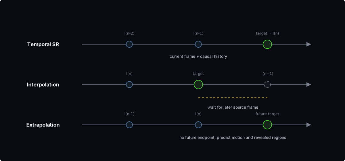
Frame generation is the broad, familiar term for synthesizing extra display frames. Within that category, interpolation and extrapolation have precise meanings. Interpolation targets a time between two source frames and uses the later endpoint. Extrapolation targets a time after the latest source frame and uses no future endpoint. A rendering-aware frame generator may also consume depth, engine motion vectors, or a separate UI surface, and may participate in the swapchain and Present, the graphics API step that submits an image for presentation. If public documentation does not establish the target timestamp, it is safer to call the operation frame generation without classifying it as interpolation or extrapolation.
Ray Reconstruction has another target. It starts from noisy or sparse ray-traced signals. In the DLSS-RR 2.12.0 integration guide, enabling Ray Reconstruction replaces the ordinary Super Resolution reconstruction stage. It is not an extra pass after SR.
1.2 Causality follows the target time
The tasks can be written in one form:
Here, τ is the target output time. Ii is an input image at time τi, and Zi contains auxiliary evidence such as motion, depth, exposure, or UI state. A method is causal with respect to the target if every Δi ≤ 0. Any Δi > 0 means that the method uses lookahead.
- Temporal SR sets τ = τn and uses samples with i ≤ n.
- Interpolation sets τn < τ < τn+1 and includes source frame n + 1.
- Extrapolation sets τ > τn while its inputs still satisfy i ≤ n.
This definition is more useful than asking which frame invokes an algorithm. Invocation time does not tell us what time the output represents, or where waiting occurs among rendering, reconstruction, queueing, and presentation.
A generation ratio only states how many frames could be inserted. The presented rate also depends on display refresh, reconstruction throughput, and the presentation queue. It says nothing by itself about simulation frequency or input sampling. A high fixed ratio can build a queue and increase latency, a risk documented in the DLSS-G 2.12.0 guide.
Target time will shape every later discussion of latency, quality, and generated-frame count. Lookahead can improve motion continuity, but the wait belongs in the interaction budget. Reporting every result as "2x FPS" erases that distinction before comparison begins.
2. Mobile system constraints
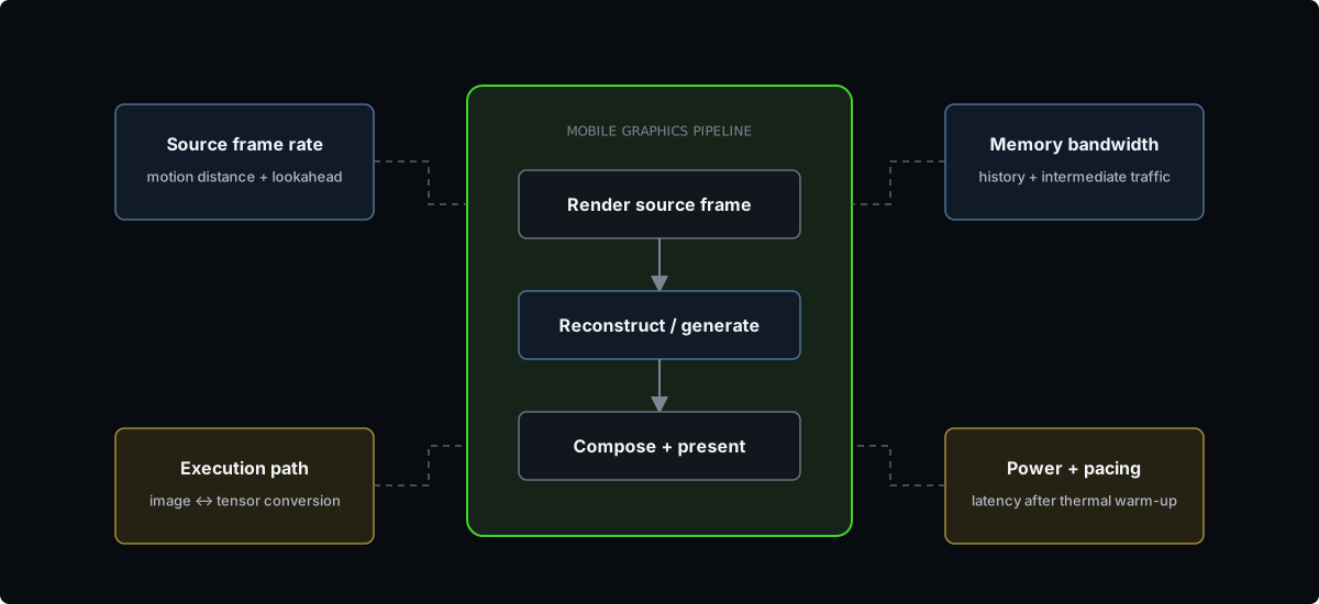
Target time determines what evidence an algorithm needs. The device determines whether that evidence can arrive within budget. Four constraints recur in mobile games:
| Constraint | Direct effect on super resolution and frame generation |
|---|---|
| Source frame rate | Longer frame intervals increase motion distance, disocclusion area, and lookahead time |
| Memory bandwidth | High-resolution history and intermediate textures may leave tile memory and be read or written every frame |
| Execution path | Transfers and format conversion between images, tensors, and execution units can erase gains from neural acceleration |
| Power and frame pacing | A short peak result does not describe sustained frame rate or interaction latency during a play session |
These constraints connect the rest of the article. Temporal accumulation consumes bandwidth. Interpolation turns the source-frame interval into lookahead latency. NSS reduces neural output, while NFRU limits full-resolution data movement. The mobile question is not whether a model can run once. It is whether reconstruction and presentation can finish repeatedly inside the device's operating envelope.
3. Temporal history, detail, and ghosting
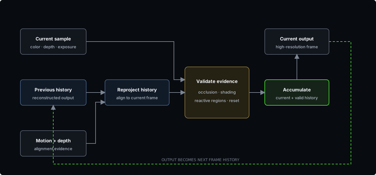
A low-resolution frame lacks more than pixel count. A thin line may fall between sample locations. Distant geometry may appear only on some frames. A low-resolution mip may already have removed texture detail. Temporal reconstruction treats successive frames as offset samples. Current color contributes new evidence, jitter changes sample positions, and history retains previously reconstructed high-resolution information.
Temporal SR is the special case of the first equation where τ = τn. Let Ŷn = Î(τn) and let Hn−1 summarize evidence from i < n. A simplified recurrence is:
Xn is current color. Zn may contain motion, depth, jitter, exposure, or material guides. Hn−1 is retained history. Rn covers camera cuts, resolution changes, and explicit resets. Nothing in this equation requires Fθ to be a neural network. FSR 2, Unreal Engine TSR, SGSR2, and Arm ASR use analytical temporal reconstruction. DLSS-SR, XeSS-SR, NSS, and MetalFX Temporal expose different amounts of their internal estimators and state.
3.1 Reproject, validate, accumulate
The system first reprojects history into the current frame using motion vectors. Depth helps resolve occlusion. Exposure places colors from different frames in a comparable range. Reactive or transparency masks identify pixels where history should not be trusted. Valid samples enter accumulation. Invalid regions fall back to current-frame evidence or a spatial reconstruction.
The same loop explains common artifacts. Incorrect motion moves old detail to the wrong place. A disoccluded region has no valid history. Transparency, particles, shadows, and reflections may not follow opaque geometry motion. A camera cut without a reset makes the entire history belong to the wrong scene. Ghosting and flicker often begin in history validation rather than model capacity.
Unreal Engine TSR documents disocclusion handling, shading rejection, flicker analysis, spatial fallback, and history resurrection. History resurrection can choose an older sample when the immediately preceding frame is a poor match. Velocity, World Position Offset, transparency, and pre-exposure feed the same history and debugging logic.
This creates a direct tradeoff. Longer or higher-resolution history can improve stability, but costs memory and bandwidth. Stronger rejection reduces ghosting, but forces details to accumulate again and can increase flicker. Temporal SR has no fixed best setting independent of content and source frame rate.
4. Interpolation and extrapolation
Temporal SR still reconstructs the present. Frame generation adds display times outside the original render cadence. The main distinction is whether a real frame after the target time is available.
Let adjacent source frames occur at τn and τn+1, separated by Tr. For a target τ = τn + αTr, an interpolation method that uses In+1 must wait:
L is only the lookahead needed to obtain future evidence. Processing, queueing, and display scanout add further delay. Extrapolation places the target after the latest source frame. It avoids waiting for a future endpoint, but must predict future motion and regions that no input has revealed.
4.1 Interpolation and lookahead
Arm NFRU is a clear example. It waits for source frames on both sides of the target, then combines engine motion vectors with block-matching optical flow to generate an intermediate image. Under uniform 30 to 60 FPS pacing, waiting for the later source frame adds half a source-frame interval of lookahead at the intermediate target time. Section 8.3 returns to its four-candidate fusion and mobile data path.
4.2 Extrapolation failure modes
GFFE studies frame extrapolation without rendering a new G-buffer. "G-buffer free" does not mean that the method needs no renderer data. It reads source color, depth, and motion vectors, but does not regenerate albedo, normals, roughness, or metallic values for the extrapolated frame.
GFFE tracks fragments in world space, predicts future positions with a linear motion model, and projects them into the future camera view. When several fragments land on one pixel, the nearest depth wins. A recurrent hierarchical background buffer fills holes left by projection. An adaptive rendering window also covers regions expected to enter the view.
Geometry alone does not update moving shadows, reflections, or other non-geometric image motion. GFFE applies a lightweight coarse-to-fine network after geometric extrapolation to correct shading. The network refines a structured prediction rather than generating the whole frame from scratch.
The paper reports a total runtime of 6.62 ms at 1080p on an RTX 4070 Ti Super with TensorRT FP16. It also passes extrapolated color, depth, and motion to DLSS 2 for super resolution. These experiments do not cover a mobile SoC, power, thermal steady state, or complete input latency.
Extrapolation removes the future-endpoint wait but adds future-motion error and background-state management. GFFE's listed limitations include never-observed internal disocclusions, UI and particles without depth, stale shading, and failures of linear motion prediction.
4.3 Interpolation, extrapolation, and SR in one framework
Mob-FGSR places these targets in one mobile framework. It consumes rendered color, depth, and engine motion vectors. Its modes include interpolation, extrapolation, temporal SR, interpolation with SR, and extrapolation with SR.
The method first derives motion at the target time. Depth-aware motion splatting preserves foreground and background priority, followed by local repair for holes around thin objects. Interpolation warps both endpoints. Extrapolation uses only the latest source frame.
The SR branch is not an unrelated upscaler appended after a complete low-resolution generated frame. It shares motion reconstruction and uses an SR-aware temporal warp to reconstruct directly at high resolution. A small MLP learns resampling weights offline and bakes them into a 32x32x16 lookup table. Runtime work consists of LUT access and shader reconstruction. The public reference uses C++/GLSL and OpenGL 4.3; it does not disclose a complete production Android integration path.
On Snapdragon 8 Gen 3, the paper reports 2.21, 1.92, 1.66, 2.34, and 1.75 ms for interpolation, extrapolation, SR, interpolation with SR, and extrapolation with SR, respectively. These are GPU processing times, not touch-to-photon latency. The Android demo uses a synthetic no-op rendering workload, and the public code does not include production presentation or UI integration. Its 110+ FPS demo result should not be generalized to ordinary games.
Interpolation has more evidence and pays for lookahead. Extrapolation avoids the future endpoint and pays in uncertainty around motion and disocclusion. Mob-FGSR also shows that SR and frame generation can share a motion front end while producing images at different target times. The right route depends on interaction budget, source frame rate, renderer signals, and acceptable failure modes, not on the advertised multiplier alone.
5. Neural reconstruction outputs
"AI upscaling" is too broad to describe an algorithm. A network may output RGB, filter parameters, candidate weights, confidence, or a local correction. A runtime with no neural network may still use a LUT learned offline. The estimator's output determines much of the data path and many of its failures.
| Estimator form | Representative routes | Runtime output | Main advantage | Main risk |
|---|---|---|---|---|
| Analytical rules | FSR 1/2/3, UE TSR, SGSR1/2, Arm ASR | Reprojection, validation, filtering, and composition | Visible stages that can be adapted to hardware | Complex rules and manually handled edge cases |
| Neural image reconstruction | DLSS-SR/RR, XeSS-SR | A high-resolution or denoised current image | Learns complicated image priors | Model, training, and state are often undisclosed |
| Neural parameter prediction | Arm NSS | Filtering and temporal-control parameters | Keeps high-resolution RGB in the graphics pipeline | Wrong parameters can still corrupt frame history |
| Candidate-weight prediction | Arm NFRU | Weights for four motion-aligned candidates | Candidate construction and composition remain explicit | No correct output exists if all candidates fail |
| Heuristic geometry with neural correction | GFFE | Shading correction after geometric extrapolation | Restricts the network to changes that rules handle poorly | Still limited by future-motion and background-history errors |
| Offline learning with a LUT | Mob-FGSR | Resampling weights from table lookup | No runtime neural network and a mobile-friendly shader path | A different scale factor requires a retrained LUT |
5.1 Analytical methods move complexity into state
FSR 2, TSR, SGSR2, and ASR all manage reprojection, history clipping, disocclusion, and fallback. SGSR2 also maintains transparency and luminance activity state. Unreal Engine TSR integrates flicker analysis, history resurrection, and content annotations. Their complexity lives in state management and explicit rules.
The benefit is inspectability. A mobile implementation can change shader type, compress intermediate color, or reduce history precision and resolution. The cost moves into rule design, material conventions, and debugging tools.
5.2 Small networks can sit at different boundaries
NSS, NFRU, and GFFE divide work in three ways. NSS uses an INT8 network to predict filtering and temporal controls. NFRU predicts weights among existing candidates. GFFE performs geometric extrapolation first and uses a small network for shading correction. Each leaves part of high-resolution image reconstruction in explicit graphics processing.
This division preserves renderer evidence and makes fallback behavior easier to define. It cannot create missing evidence. If motion, occlusion, or history is already wrong, restricting neural output changes the form and extent of the error, not the underlying information limit.
5.3 Public inputs do not reveal internal design
Public DLSS, XeSS, and MetalFX material describes required inputs and integration behavior without publishing complete models, training procedures, or history representations. Those sources support comparisons of target time, required resources, pipeline placement, platform scope, and control over UI or Present. Similar inputs do not support claims about model architecture or technical lineage.
MetalFX and FSR expose overlapping spatial and temporal roles, along with inputs such as color, depth, motion, and jitter. Their public material establishes neither derivation nor code reuse. Similar interfaces can support the same renderer task without sharing an implementation lineage.
6. System responsibilities in PC suites
PC suites provide a useful system map. Temporal upscaling owns current-frame history. Frame generation inserts additional images into the display path. Latency control manages when CPU and GPU work is submitted. Newer runtimes also change what the reconstruction stage produces and how its model is distributed. DLSS, FSR, and XeSS are examples of these responsibilities rather than the organizing taxonomy.
6.1 History enters current-frame reconstruction
A spatial upscaler reads one image. A temporal upscaler also consumes previous output, which requires motion, occlusion, jitter, exposure, and reset policy. A reusable model therefore depends on a stable renderer contract as much as on training.
Early NVIDIA DLSS required training for each game. DLSS 2 introduced a generalized model that combined low-resolution color and motion vectors with the previous high-resolution output. AMD moved from FSR 1 spatial scaling to FSR 2 analytical temporal reconstruction. Intel XeSS 1.x began as AI temporal supersampling. Their estimators differ, but history introduces the same classes of failure.
6.2 Frame generation reaches Present
DLSS 3 added one generated frame and bundled Reflex with the suite. The first DLSS Frame Generation route used sequential game frames, hardware optical flow, engine motion vectors, and depth. NVIDIA's 2025 DLSS 4 description states that the then-current model replaced this earlier hardware-optical-flow route, so the 2022 mechanism should not be generalized to current versions.
FSR 3 and XeSS 2 also package super resolution, frame generation, and low-latency control. FSR 3.1 decoupled analytical frame generation from the upscaler, allowing it to run with another upscaler or native-resolution rendering.
Frame generation reaches Present, the graphics API operation that submits an image to the presentation system. Where generated frames enter that path, how UI is composed, how deep the queue becomes, and where CPU or GPU work waits all affect latency. Super resolution, frame generation, and latency control can cooperate, but evaluation should still report them separately.
6.3 Models and runtimes change the output boundary
Later PC suites changed several boundaries in parallel. DLSS 3.5 introduced Ray Reconstruction for ray-traced signals. DLSS 4 added Multi Frame Generation, and Dynamic MFG adjusts generation count against a target rate or display refresh. DLSS 5 then extended neural rendering to lighting and materials. NVIDIA announced it as a preview planned for fall 2026, with final hardware support, memory use, and performance cost still unpublished.
Distribution changed too. XeSS 3 added 3x and 4x modes on Intel Arc hardware. AMD's FSR 4.x distributes ML super resolution and frame generation through signed runtimes, while the analytical FSR 1, 2, and 3 implementations publish source. A stable API does not imply that the model is public, which affects customization, updates, and validation.
7. History and presentation ownership
An engine, system framework, vendor runtime, or application can own the same temporal reconstruction slot. Ownership determines who defines history, triggers resets, inspects failures, and replaces components.
7.1 Engine ownership: Unreal Engine TSR
Unreal Engine 5.7 places TAAU, TSR, DLSS, FSR, and XeSS at the same temporal-upscaler point. The engine owns TSR history, disocclusion, shading rejection, flicker analysis, and fallback. Information from material animation and transparency also affects history decisions.
This coupling gives the engine access to intermediate state and content-aware debugging. It also ties quality to renderer conventions. Epic's platform matrix does not list TSR for the stock mobile forward or deferred paths, so TSR is used here as a desktop and console example of engine-owned reconstruction, not as a stock mobile route.
7.2 System framework ownership: Apple MetalFX
MetalFX encapsulates history and device variation in a system framework. Its Spatial scaler reads the current antialiased color image. Its Temporal scaler combines color, depth, motion, jitter metadata, and internally retained history to reconstruct the current frame. WWDC22 MetalFX
The application does not provide an explicit history-color texture. It can request a reset, but cannot inspect the estimator, training process, execution unit, or internal history representation. MetalFX documentation shows the integration surface, not the scaler implementation. Newer MetalFX APIs list frame interpolation and temporal denoised scaling as separate effects. They should not be conflated with the original Temporal scaler.
7.3 Vendor runtimes and application pipelines
Vendor runtimes own the central DLSS and XeSS estimators, while the application supplies images and renderer state. Analytical FSR and SGSR expose more shader code and intermediate state, which platforms can modify directly. Runtime ownership makes vendor model updates easier. Application ownership leaves more room to adapt precision, synchronization, and data residency.
Frame generation extends that control toward Present because UI composition, queue depth, and pacing affect the displayed result. FSR 3.1's separation of upscaling and frame generation shows that the components can cooperate while remaining replaceable and independently measurable. On mobile, access to intermediate stages determines how much room remains to reduce bandwidth or synchronization cost.
8. Mobile reconstruction pipelines
Mobile adaptation is not a desktop model recompiled at a smaller size. Tile-based GPUs try to keep intermediate values on chip. Full-resolution history, extra textures, format conversion, and synchronization can force data into external memory. A method with modest arithmetic may still lose time to bandwidth or queueing. The data path often changes before the model does.
8.1 From spatial scaling to temporal reconstruction
Qualcomm SGSR1 reads the current image and performs spatial upscaling and sharpening in one shader pass. It needs no history and has a simple integration contract. It also cannot use adjacent frames to recover detail.
SGSR2 is a separate temporal route. It adds motion, depth, jitter, exposure, and previous output. The public implementation provides fragment and compute variants with different pass counts and history state. Some paths fit more naturally into tile rendering. Others compress intermediate color or spend extra history on transparency and activity detection. They solve the same reconstruction task through different memory paths.
Arm ASR 25.06 starts from the analytical temporal framework in FSR 2.2.2. It moves more work to fragment shaders, uses explicit 16-bit types, and exposes several quality presets. Both SGSR2 and ASR reconsider which evidence to retain, what precision to use, and where intermediate values should live.
8.2 NSS: Predicting controls instead of pixels
Arm Neural Super Sampling reconstructs the current high-resolution frame. It uses current color, motion, depth, and history, but its network predicts local filtering and temporal controls. Shaders produce the final RGB image. This division follows mobile constraints rather than a preference for one model style.
Arm's walkthrough compares three options. Direct image prediction offers the most freedom, but INT8 quantization produced color shifts, over-sharpening, and banding, especially for HDR. Predicting a complete filter kernel quantized more reliably. It also produced too much data: a per-pixel 3x3 kernel for a 1080p image requires nine coefficients per output pixel, followed by another read to apply the filter. Neural compute had become a bandwidth problem.
NSS instead predicts fewer controls. An accumulation parameter determines how quickly new samples enter history. Rectification controls decide when stale history should be clipped. Targeted filter weights operate on the aliased current sample. The model also carries hidden state across frames and reads temporal luminance change, which helps distinguish thin features sampled intermittently by jitter from stale history.
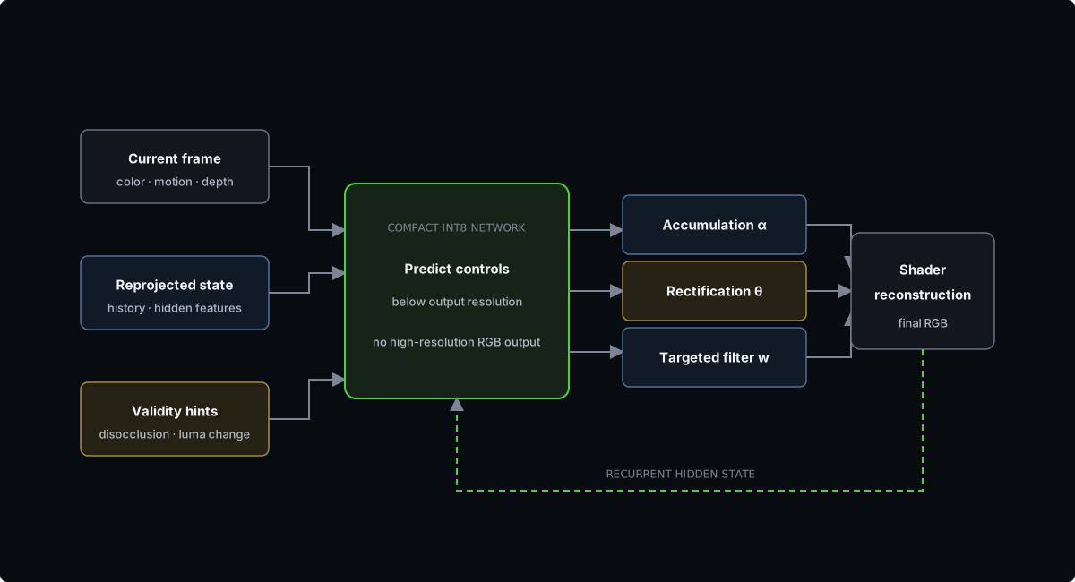
This deliberately limits the network's responsibility. Controls can be predicted below output resolution, while graphics passes handle motion, history reprojection, current-sample filtering, and final accumulation. The network still handles local decisions that are difficult to encode by hand, but high-resolution color does not need to travel through it. Arm's public NSS material provides feasibility estimates based on target latency, shader cost, and assumed accelerator efficiency. It does not provide a reproducible production-phone benchmark for this article, so no production timing is claimed here.
8.3 NFRU: preserve candidates, then learn the blend
Arm Neural Frame Rate Upscaling targets an intermediate time. It waits for rendered frames on both sides. Under the 30 to 60 FPS cadence shown by Arm, this introduces half a source-frame interval of lookahead at the target. Processing, queueing, and display add more to touch-to-photon latency.
Interpolation first needs motion. Engine vectors describe geometry well, but omit moving shadows, reflections, and many particles. Image-based optical flow can observe those appearance changes, but is less reliable around occlusion and low-texture regions. NFRU does not force both motion sources into one field. It warps the earlier and later frames with each source, producing four candidate images.
Those candidates retain complementary evidence. A region missing from the earlier frame may be visible in the later one. Optical flow may capture a moving shadow that geometry motion misses. Depth and disocclusion signals act as reliability hints rather than unquestioned truth. An INT8 network predicts per-pixel blend weights, and a shader combines the four floating-point candidate colors. Small weight errors remain mixtures of available image evidence instead of newly generated RGB values.
The candidates still create a data-movement problem. A scatter writes each source sample forward to its predicted target position; doing this with full-resolution color requires atomic operations and leaves holes. NFRU scatters only motion at lower resolution, repairs holes with depth-aware dilation, then gathers color by reading the source location for each output pixel. Motion processing and neural inference remain at a lower internal resolution. Only the final color sampling scales with output size. This separation explains why neural throughput and operation count alone cannot predict mobile performance.
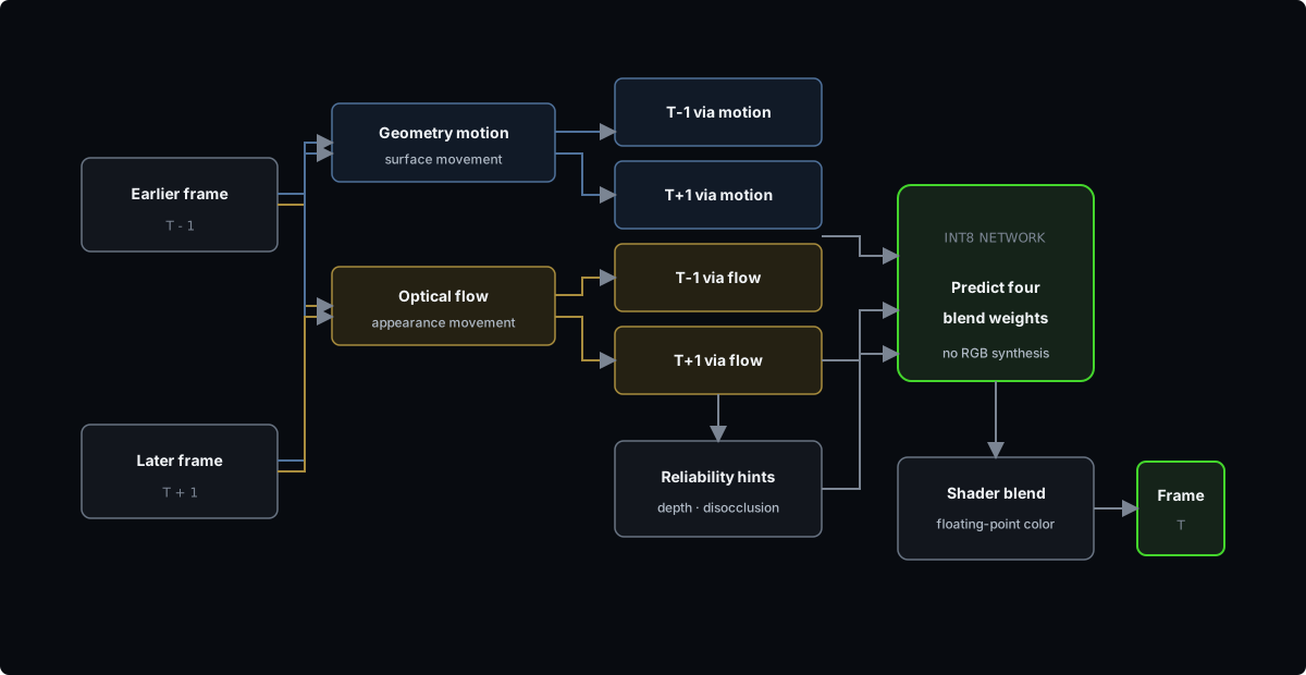
NFRU assumes approximately linear motion between source frames. A rapidly accelerating or turning object may not occupy its true intermediate position. Yet a position that is slightly early or late can look plausible in motion while receiving a large pixel error against one reference frame. Frame-generation evaluation must therefore include full-sequence viewing.
8.4 Bandwidth, pacing, and sustained performance
The Khronos Vulkan performance samples cover attachment load and store behavior, subpasses, and pipeline barriers on specific devices. Their broader lesson applies here: unnecessary stores, intermediate data leaving a tile, and barriers with excessive scope can cost more than a small amount of arithmetic. NSS reduces network output dimensionality. NFRU separates motion scatter from color gather. Both are responses to this cost structure.
After reconstruction, a frame still passes through system composition and display queues. AOSP graphics architecture explains how an old buffer may be reused when no new content arrives. Android Frame Pacing uses presentation timestamps and fences to control cadence. Submitting more frames does not guarantee that the display presents them at the same rate. A deep queue can instead increase latency.
Power and temperature complete the mobile budget. The Android Thermal API documentation states that a device can sustain peak performance only for a limited time. A useful game benchmark should report source render rate, presented rate, latency, power, and frame time after thermal warm-up. A short cold-device peak does not show whether the method can last through a play session.
9. Data must match the target time
Temporal SR and frame generation cannot share an ambiguous collection of "video data." Temporal SR needs a low-resolution input and high-resolution reference for the same target time. Interpolation needs an image rendered at the intermediate time. Extrapolation needs a retained future target to measure prediction error. Analytical methods do not need training data, but their tests still need the correct temporal relation.
9.1 NSS: input and reference from one render
NSS data generation begins with one high-resolution render. The Arm walkthrough derives both the antialiased reference and jittered low-resolution input from that result. Geometry, lighting, and screen-space effects therefore remain aligned. The important point is not the particular 8K source size. Input and reference do not come from independent renders, where random particles, SSAO, or resolution-dependent effects could corrupt supervision.
NSS must learn convergence across frames as well as spatial reconstruction. Training runs several temporal steps, then backpropagates through those steps. Its loss compares both spatial quality and reprojected temporal change. L1 and LPIPS terms favor agreement with the current reference. Temporal terms penalize instability across frames. Arm treats temporal stability and spatial fidelity as competing objectives, which mirrors the runtime tradeoff in history accumulation.
9.2 NFRU: source frames and intermediate truth use different cadences
NFRU targets a time between source frames, so its data follows that timing. Arm's training procedure captures the same deterministic content at 60 FPS and 30 FPS. The high-rate sequence supplies the true intermediate image. The low-rate sequence supplies motion vectors with the same interval as the runtime source frames. This is a task-specific construction for 30 to 60 FPS interpolation, not a universal recipe for video interpolation data.
Even this dataset does not imply a unique perceptual answer. NFRU assumes nearly linear motion, while real objects accelerate and turn. A prediction can be a little early or late, look natural in playback, and still produce a large pixel error. PSNR, SSIM, and LPIPS can detect regressions, but cannot replace watching the sequence.
Dataset size does not replace failure coverage. Fast motion, thin geometry, particles, shadows, transparency, disocclusion, exposure changes, and camera cuts arise from different causes. A ghost may come from reversed motion, stale history, or failed occlusion logic. With camera and object paths fixed, changing motion, resetting history, or removing an occlusion hint isolates those causes more effectively than adding similar frames.
Data should be split before derived samples are generated. Adjacent frames, patches, and interpolation tuples from one capture are highly correlated. Randomly splitting them afterward can place near-duplicates of the same motion in training and validation. Gotz-Hahn et al. studied leakage in a video-quality pipeline, not reconstruction training, but the conservative implication transfers: group by source scene or capture first, verify no group overlap, then derive samples.
9.3 From image quality to end-to-end experience
Single-frame metrics answer how far one aligned image is from a reference. PSNR, SSIM, LPIPS, and FLIP can measure spatial error, but do not show ghosting accumulating across frames or whether generated frames reach the display at the intended cadence.
Temporal metrics relate neighboring frames. FloLPIPS, TecoGAN's temporal metrics, and masked warping error measure different forms of inconsistency. Their flow estimator, warp direction, masks, value range, normalization, and pooling are part of the metric definition. A low warping error may also reward excessive blur. Spatial metrics, temporal metrics, and full-sequence viewing must be interpreted together.
Mobile devices add a third layer: whether frames arrive on time and whether performance lasts. Platform timestamps can expose presentation intervals, missed deadlines, and dropped frames, but they do not directly measure photons from the display. Thermal status is not electrical power measurement. ITU-T P.910 defines procedures for non-interactive one-way video quality, not game input response. A complete comparison observes image quality, pacing, touch-to-photon latency, power, and thermal steady state during representative play.
10. Synthesis: Choose the time, then trace the data
Start with the target time and acceptable lookahead. That choice determines whether the system needs current history, a later source frame, or a prediction beyond the latest render. Next, identify the renderer evidence needed to handle motion and disocclusion. Only then trace history, candidates, format conversions, and external-memory traffic through the device, and check whether latency remains stable after thermal warm-up.
NSS and NFRU reach different answers because they target different times. NSS reconstructs the present and spends its compact neural output on filtering and history control. NFRU reconstructs the interval, preserves four motion-aligned candidates, and accepts the wait for the later source frame. Their models matter, but the target time and data path explain why each model has the job it does.
References
PC vendor suites
- NVIDIA, Streamline v2.12.0 programming guides.
- Kilgariff et al., NVIDIA Turing Architecture In-Depth, 2018.
- NVIDIA, DLSS 2.0: A Big Leap In AI Rendering, 2020.
- NVIDIA, DLSS 3, 2022.
- NVIDIA, DLSS 3.5 Ray Reconstruction, 2023.
- NVIDIA, DLSS 4, 2025.
- NVIDIA, DLSS 4.5 Dynamic MFG and 6X availability, 2026.
- NVIDIA, DLSS 5 Delivers AI-Powered Breakthrough In Visual Fidelity For Games, 2026.
- AMD GPUOpen, FSR 1, FSR 2, and FSR 3.
- AMD GPUOpen, FidelityFX SDK v2.3.0, 2026.
- Intel, XeSS-SR, XeSS-FG, and XeLL, SDK 3.0.2.
Engines, platforms, and mobile methods
- Epic Games, Temporal Super Resolution and Temporal Upscalers, Unreal Engine 5.7.
- Apple, MetalFX and Boost performance with MetalFX Upscaling.
- Qualcomm, Snapdragon Game Super Resolution and SGSR2.
- Arm, Accuracy Super Resolution 25.06.
- Arm, Neural Super Sampling and Neural Graphics Model Gym.
- Arm, Mobile Neural Frame Rate Upscaling and Neural Graphics SDK.
- Android, Frame Pacing, Thermal API, and SurfaceFlinger/HWC.
- Khronos, Vulkan performance samples.
Academic frame generation and reconstruction
- Wu et al., GFFE: G-buffer Free Frame Extrapolation for Low-latency Real-time Rendering, ACM TOG / SIGGRAPH Asia 2024.
- Yang et al., Mob-FGSR: Frame Generation and Super Resolution for Mobile Real-Time Rendering, SIGGRAPH 2024.
- Yang et al., Mob-FGSR project and code.
Evaluation
- ITU-T, P.910 (10/23).
- Andersson et al., FLIP, 2020.
- Danier et al., FloLPIPS, 2022.
- Chu et al., TecoGAN temporal metrics, 2020.
- Lai et al., Learning Blind Video Temporal Consistency, 2018.